In [1]:
%%html
<script>
code_show=true;
function code_toggle() {
 if (code_show){
 $('div.input').hide();
 } else {
 $('div.input').show();
 }
 code_show = !code_show
}
$( document ).ready(code_toggle);
</script>
<a href="#" onClick="code_toggle();"><h3>Click here to hide/show the code</h3></a>
A tour of point cloud processing
Mathieu Carette
Notebook available at https://github.com/rockestate/point-cloud-processing
Slides available at https://www.rockestate.be/point-cloud-processing/presentation/
(previous versions here)
About me
- PhD in Mathematics (ULB, 2009)
- Postdocs (UIUC, UCLouvain, McGill)
- Data Scientist (KBC, Forespell)
- Now working on

ROCKESTATE
Favorite software stack:
Where do 3D point clouds come from?
In [2]:
from IPython.display import YouTubeVideo
YouTubeVideo('GSPcyhSAgTQ',start=7, end=31)
Out[2]:
Open LiDAR data for Brussels and Flanders : https://remotesensing.agiv.be/opendata/lidar/
- PCL Point Cloud Library
- Open source: https://github.com/PointCloudLibrary/pcl
- C++
- Powerful general purpose algorithms
- CGAL Computational Geometry Algorithms Library
- Open source: https://github.com/CGAL/cgal
- C++
- State of the art 2D and 3D geometry algorithms
- PDAL Point Data Abstraction Library
- Open source: https://github.com/PDAL/PDAL
- C++, command-line, python
- Wraps some PCL functionality
- For windows users: part of the OSGeo4W distribution
- LAStools from RapidLasso
- Proprietary, preferred pricing for academic use
- Windows only, runs on wine
- command-line, GUI
- Open source laszip compression/decompression: https://github.com/LASzip/LASzip
Let's process some point clouds
In [3]:
import glob
import io
import ipyleaflet
import IPython.display
import ipyvolume.pylab as p3
import json
import matplotlib.cm
import matplotlib.pyplot as plt
import numpy as np
import os
import pandas as pd
import pdal
import PIL
import pyproj
import requests
import shapely.geometry
import scipy.spatial
import sys
import urllib.request

%load_ext autoreload
%autoreload 2

sys.path.append('../src')
from pcl_utils import local_max

# Url for aerial imagery
IVaerial = "https://geoservices.informatievlaanderen.be/raadpleegdiensten/ogw/wms?SERVICE=WMS&VERSION=1.3.0&REQUEST=GetMap&CRS=EPSG:31370&BBOX={0},{1},{2},{3}&WIDTH=512&HEIGHT=512&LAYERS=OGWRGB13_15VL&STYLES=default&FORMAT=image/png"

%matplotlib inline
In [4]:
# Download the LAS data file if not already present
if not os.path.isdir('../data'):
    os.makedirs('../data')
lidar_filename = 'LiDAR_DHMV_2_P4_ATL12431_ES_20140325_31195_2_150500_166500.las'
if not os.path.isfile('../data/' + lidar_filename):
    urllib.request.urlretrieve('https://s3-eu-west-1.amazonaws.com/rockestate-public/lidar/' + lidar_filename,
                               '../data/' + lidar_filename)
In [ ]:
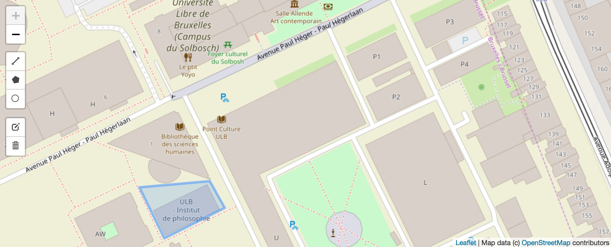
m = ipyleaflet.Map(center=(50.81343, 4.38188), zoom=16)
dc = ipyleaflet.DrawControl()
m.add_control(dc)
m
Selecting street portion with a polygon
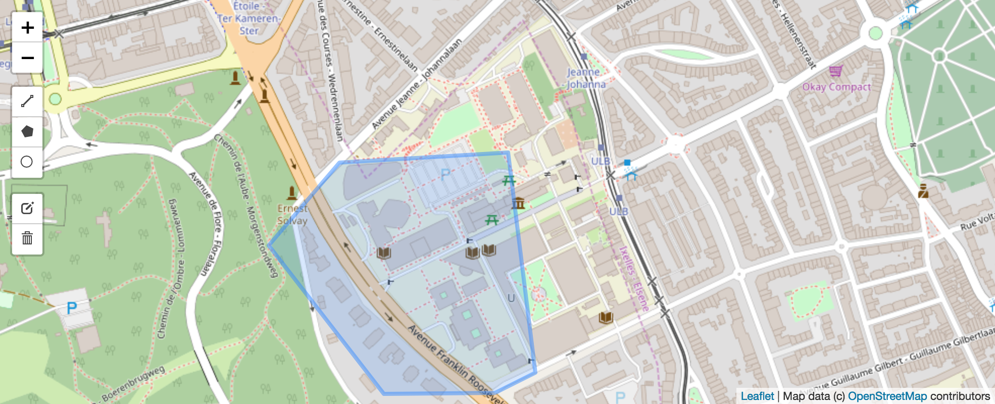
In [6]:
wsg84 = pyproj.Proj(init='epsg:4326')
lambert = pyproj.Proj(init='epsg:31370')
coords = [pyproj.transform(wsg84,lambert,x,y) for (x,y) in dc.last_draw['geometry']['coordinates'][0]]
polygon = shapely.geometry.Polygon(coords)
print(polygon.wkt)
IPython.display.display(polygon)
In [7]:
b = polygon.bounds
cropper = {
    "pipeline": [ '../data/'+ lidar_filename,
        {   "type":"filters.crop",
            'bounds':str(([b[0], b[2]],[b[1], b[3]]))},
        {   "type":"filters.crop",
            'polygon':polygon.wkt},
        {   "type":"filters.hag"},
        {   "type":"filters.eigenvalues",
            "knn":16},
        {   "type":"filters.normal",
            "knn":16}
    ]}
pipeline = pdal.Pipeline(json.dumps(cropper))
pipeline.validate()
%time n_points = pipeline.execute()
print('Pipeline selected {} points ({:.1f} pts/m2)'.format(n_points, n_points/polygon.area))
In [8]:
# Load Pipeline output in python objects
arr = pipeline.arrays[0]
description = arr.dtype.descr
cols = [col for col, __ in description]
df = pd.DataFrame({col: arr[col] for col in cols})
df['X_0'] = df['X']
df['Y_0'] = df['Y']
df['Z_0'] = df['Z']
df['X'] = df['X'] - df['X_0'].min()
df['Y'] = df['Y'] - df['Y_0'].min()
df['Z'] = df['Z'] - df['Z_0'].min()
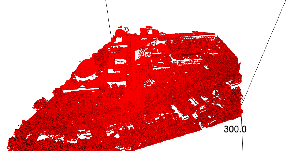
In [ ]:
fig = p3.figure(width=1000)
fig.xlabel='Y'
fig.ylabel='Z'
fig.zlabel='X'
all_points = p3.scatter(df['Y'], df['Z'], df['X'], color='red', size=.2)
p3.squarelim()
p3.show()
Original data
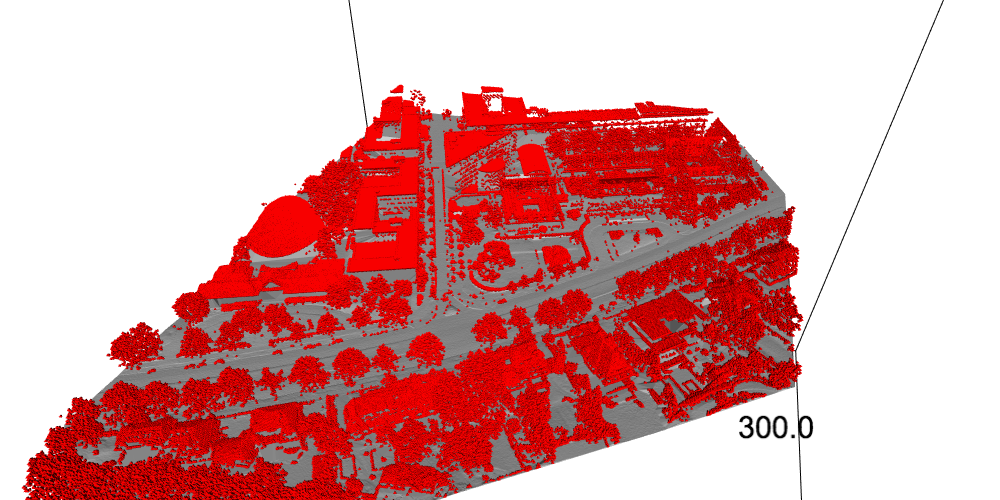
In [10]:
# Color ground in grey
df['ground'] = df['Classification']!=1
ground = p3.scatter(df.loc[df['ground'],'Y'], df.loc[df['ground'],'Z'], df.loc[df['ground'],'X'], color='red', size=.2)
non_ground = p3.scatter(df.loc[~df['ground'],'Y'], df.loc[~df['ground'],'Z'], df.loc[~df['ground'],'X'], color='red', size=.2)
fig.scatters.append(ground)
fig.scatters.append(non_ground)
all_points.visible = False
ground.color='lightgrey'
In [11]:
# Show ground as surface
ground_delaunay = scipy.spatial.Delaunay(df.loc[df['ground'],['X','Y']])
ground_surf = p3.plot_trisurf(df.loc[df['ground'],'Y'], df.loc[df['ground'],'Z'], df.loc[df['ground'],'X'], ground_delaunay.simplices, color='lightgrey')
fig.meshes.append(ground_surf)
ground.visible=False
Use gound / non-ground classification
In [12]:
# Color points according to flatness
df['flatness'] = df['Eigenvalue0']
non_ground.color=matplotlib.cm.viridis(df.loc[~df['ground'],'flatness']*4)[:,0:3]
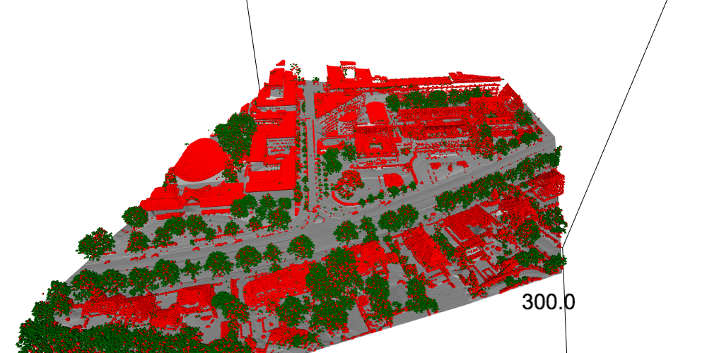
In [13]:
# Separate between trees and the rest
df['tree_potential'] = (df['Classification']==1) & (df['HeightAboveGround'] >= 2) & (df['flatness'] > .05) & (df['NumberOfReturns'] - df['ReturnNumber'] >= 1)
df['other'] = ~df['ground'] & ~df['tree_potential']
tree_potential = p3.scatter(df.loc[df['tree_potential'],'Y'], df.loc[df['tree_potential'],'Z'], df.loc[df['tree_potential'],'X'], color=matplotlib.cm.viridis(df.loc[df['tree_potential'],'flatness']*4)[:,0:3], size=.2)
other = p3.scatter(df.loc[df['other'],'Y'], df.loc[df['other'],'Z'], df.loc[df['other'],'X'], color=matplotlib.cm.viridis(df.loc[df['other'],'flatness']*4)[:,0:3], size=.2)
non_ground.visible=False
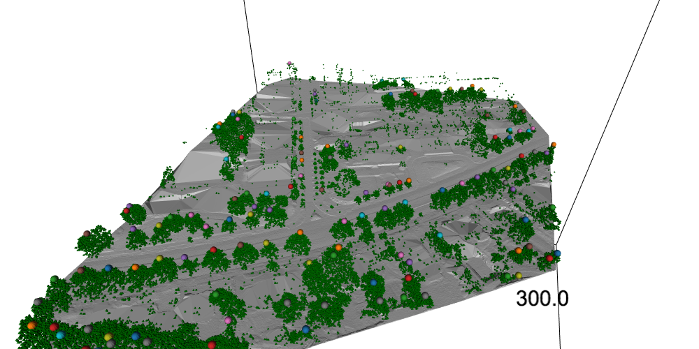
tree_potential.color='darkgreen'
other.color='red'
Use point flatness to separate trees from the rest
In [14]:
#Hide non-tree
other.visible=False
In [15]:
lep = local_max(df.loc[df['tree_potential'],['X','Y','Z','HeightAboveGround']], radius=3, density_threshold=15)
In [16]:
treetop_spheres = p3.scatter(lep['Y'], lep['Z'], lep['X'], color='red', size=.5, marker='sphere')
fig.scatters.append(treetop_spheres)
In [17]:
treetop_spheres.color = matplotlib.cm.Vega10(np.arange(len(lep['Z']))%10)[:,0:3]
Find treetops as local maxima
In [18]:
kdtree = scipy.spatial.kdtree.KDTree(lep[['X','Y','Z']])
dist, idx = kdtree.query(df.loc[df['tree_potential'],['X','Y','Z']].values)
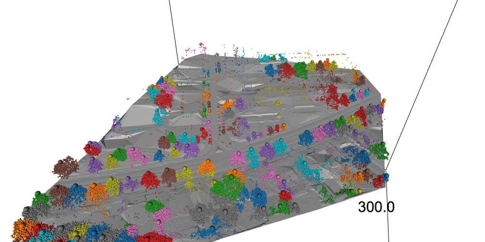
tree_potential.color=matplotlib.cm.Vega10(idx%10)[:,0:3]
df.loc[df['tree_potential'], 'tree_idx'] = idx
Separate trees using closest treetop
In [19]:
medians = df.groupby('tree_idx')[['X','Y','Z']].median()
for axis in ['X','Y','Z']:
    df['d'+axis] = df[axis] - df['tree_idx'].map(medians[axis])
df['radius'] = np.linalg.norm(df[['dX', 'dY', 'dZ']].values, axis=1)
radii = pd.DataFrame([df.groupby('tree_idx')['radius'].quantile(.5), lep['HeightAboveGround'].values*.4]).min()
In [20]:
scale = max(df['X'].max() - df['X'].min(), df['Y'].max() - df['Y'].min())
treetop_spheres.x = medians['Y']
treetop_spheres.y = medians['Z']
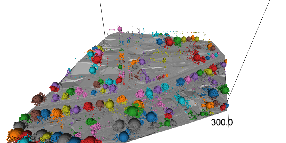
treetop_spheres.z = medians['X']
treetop_spheres.size = radii * 100 / scale
Model each tree individually
In [21]:
tree_potential.visible = False
In [22]:
other.visible = True
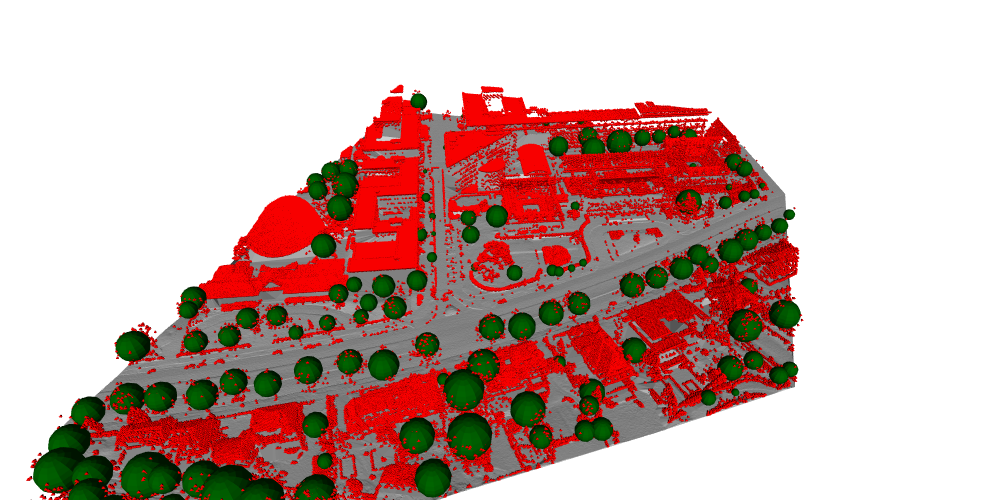
treetop_spheres.color='darkgreen'
p3.style.use('minimal')
Final street model
Building Modeling
In [ ]:
m2 = ipyleaflet.Map(center=(50.81343, 4.38188), zoom=17)
dc2 = ipyleaflet.DrawControl()
m2.add_control(dc2)
m2
Selecting building with a polygon
In [24]:
wsg84 = pyproj.Proj(init='epsg:4326')
lambert = pyproj.Proj(init='epsg:31370')
coords = [pyproj.transform(wsg84,lambert,x,y) for (x,y) in dc2.last_draw['geometry']['coordinates'][0]]
polygon2 = shapely.geometry.Polygon(coords)
print(polygon2)
IPython.display.display(polygon2)
In [25]:
b = polygon2.bounds
cropper = {
    "pipeline": list(glob.glob('../data/*150500_166500.las')) + [ # [ '../data/' + lidar_filename,
        {   "type":"filters.crop",
            'bounds':str(([b[0], b[2]],[b[1], b[3]]))},
        {   "type":"filters.merge"},
        {   "type":"filters.hag"},
        {   "type":"filters.crop",
            'polygon':polygon2.wkt},
        {   "type":"filters.eigenvalues",
            "knn":16},
        {   "type":"filters.normal",
            "knn":16}
    ]}
pipeline = pdal.Pipeline(json.dumps(cropper))
pipeline.validate()
%time n_points = pipeline.execute()
print('Pipeline selected {} points ({:.1f} pts/m2)'.format(n_points, n_points/polygon2.area))
In [26]:
arr = pipeline.arrays[0]
description = arr.dtype.descr
cols = [col for col, __ in description]
df = pd.DataFrame({col: arr[col] for col in cols})
df['X_0'] = df['X']
df['Y_0'] = df['Y']
df['Z_0'] = df['Z']
df['X'] = df['X'] - df['X_0'].mean()
df['Y'] = df['Y'] - df['Y_0'].mean()
df['Z'] = df['Z'] - df['Z_0'].min()
df.loc[df['HeightAboveGround'] < .2,'Classification'] = 2
In [ ]:
fig = p3.figure(width=1000)
fig.xlabel='Y'
fig.ylabel='Z'
fig.zlabel='X'
ground_delaunay = scipy.spatial.Delaunay(df.loc[df['Classification'] != 1, ['X','Y']])
ground = p3.plot_trisurf(df.loc[df['Classification'] != 1,'Y'], df.loc[df['Classification'] != 1,'Z'], df.loc[df['Classification'] != 1,'X'], triangles = ground_delaunay.simplices, color='lightgrey')
non_ground = p3.scatter(df.loc[df['Classification'] == 1,'Y'], df.loc[df['Classification'] == 1,'Z'], df.loc[df['Classification'] == 1,'X'], color='red', size=.2)
p3.squarelim()
p3.show()
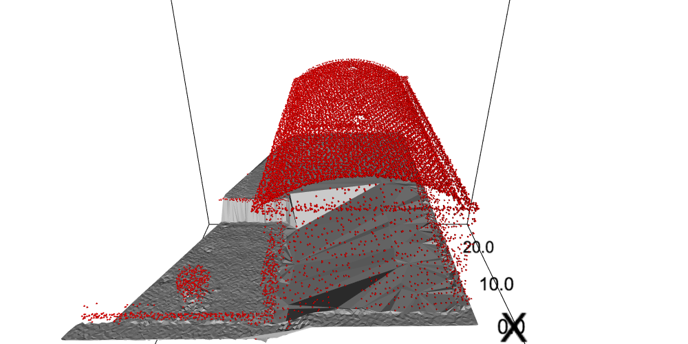
Original data
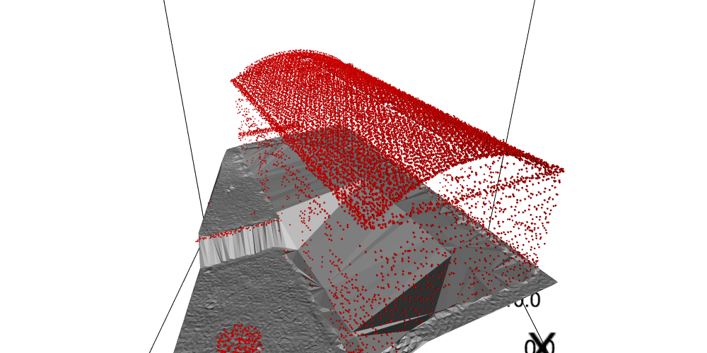
In [28]:
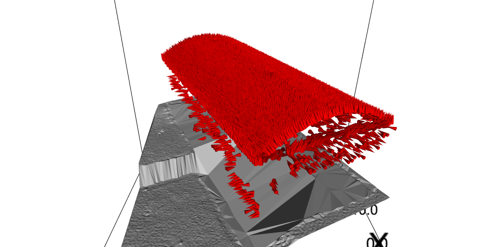
roof_mask = (df['Classification'] == 1) & (df['HeightAboveGround'] > 7) & (df['Eigenvalue0'] <= .02) & (df['NumberOfReturns'] == df['ReturnNumber'])
In [29]:
roof_quiver = p3.quiver(df.loc[roof_mask,'Y'],df.loc[roof_mask,'Z'],df.loc[roof_mask,'X'], df.loc[roof_mask,'NormalY'], df.loc[roof_mask,'NormalZ'], df.loc[roof_mask,'NormalX'], size=2)
fig.scatters.append(roof_quiver)
non_ground.visible=False
Visualize normals
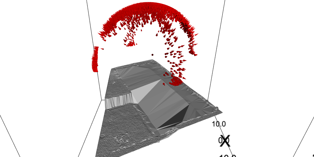
In [30]:
roof_quiver.x = df.loc[roof_mask,'NormalY'] *15
roof_quiver.y = df.loc[roof_mask,'NormalZ'] *15 + df['Z'].median()
roof_quiver.z = df.loc[roof_mask,'NormalX'] *15
Infer building orientation using normals
In [31]:
roof_quiver.visible = False
non_ground.visible = True
In [32]:
# Find building orientation using normals
alphas = np.linspace(0, np.pi, num=180)
magnitude = [np.abs(df.loc[roof_mask,['NormalX','NormalY']].values @ np.array([np.cos(alpha), np.sin(alpha)])).sum()
             for alpha in alphas]
angle = alphas[np.argmin(magnitude)]
In [33]:
# Rotate building to align walls with X & Y axes
Rotation = np.array([[np.cos(angle), np.sin(angle)],[-np.sin(angle), np.cos(angle)]])
df['X_r'], df['Y_r'] = (df[['X','Y']].values @ Rotation[i] for i in (0,1))
df['NormalX_r'], df['NormalY_r'] = (df[['NormalX','NormalY']].values @ Rotation[i] for i in (0,1))
ground.x, ground.z = df.loc[df['Classification']!= 1, 'Y_r'], df.loc[df['Classification']!= 1, 'X_r']
non_ground.x, non_ground.z = df.loc[df['Classification']== 1, 'Y_r'], df.loc[df['Classification']== 1, 'X_r']
Align building orientation along X-Y axes
In [34]:
# Build 3D model in rotated coordinates
z0 = df.loc[~roof_mask,'Z'].median()
ystep = (df.loc[roof_mask,'Y_r']*4).astype(int)/4
y_profile = (df[roof_mask].groupby(ystep)['Z'].quantile(.99).rolling(window=5).min()).shift(-1).fillna(z0)
xstep = np.linspace(df.loc[roof_mask,'X_r'].quantile(.01), df.loc[roof_mask,'X_r'].quantile(.99), len(ystep.unique()))
X,Y = np.meshgrid(xstep, ystep.sort_values().unique())
Z = y_profile[Y.ravel()].values.reshape(Y.shape)
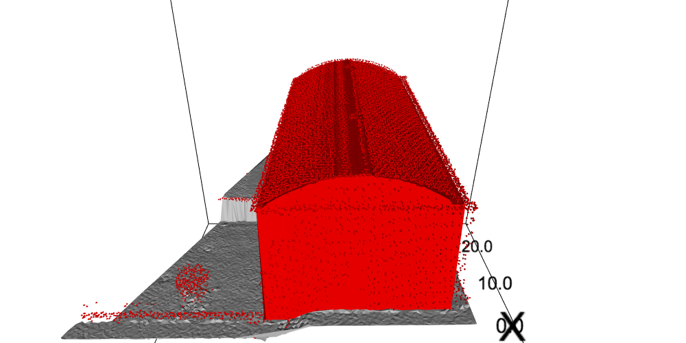
In [35]:
# Plot 3D model
df_extra = pd.DataFrame({'X_r':X.ravel(),'Y_r':Y.ravel(),'Z': Z.ravel()})
df_extra.loc[df_extra['X_r'] == df_extra['X_r'].max(), 'Z'] = z0
df_extra.loc[df_extra['X_r'] == df_extra['X_r'].min(), 'Z'] = z0
roof_delaunay = scipy.spatial.Delaunay(df_extra[['X_r','Y_r']])
roof_model = p3.plot_trisurf(df_extra['Y_r'],df_extra['Z'],df_extra['X_r'], triangles=roof_delaunay.simplices, color='red')
fig.meshes.append(roof_model)
Model the building using axis-aligned view
In [36]:
# Go back to original coordinates
df_extra['X'], df_extra['Y'] = (df_extra[['X_r','Y_r']].values @ np.linalg.inv(Rotation)[i] for i in (0,1))
df_extra['Classification'] = 6
ground.x, ground.z = [df.loc[df['Classification']!= 1, axis] for axis in ['Y','X']]
non_ground.visible=False
roof_model.x, roof_model.z = df_extra['Y'], df_extra['X']
Rotate back to original coordinate system
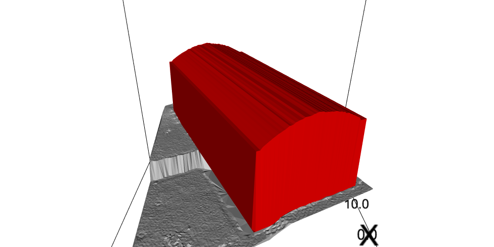
In [37]:
# Add texture to the ground
response = requests.get(IVaerial.format(*b))
texture = PIL.Image.open(io.BytesIO(response.content))
ground.u = (df.loc[df['Classification'] != 1, 'X_0'] - b[0]) / (b[2] - b[0])
ground.v = (df.loc[df['Classification'] != 1, 'Y_0'] - b[1]) / (b[3] - b[1])
ground.texture = texture
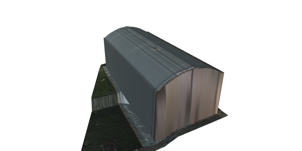
In [38]:
# ... and to the building
df_extra['X_0'] = df_extra['X'] + df['X_0'].mean()
df_extra['Y_0'] = df_extra['Y'] + df['Y_0'].mean()
roof_model.u = (df_extra['X_0'] - b[0]) / (b[2] - b[0])
roof_model.v = (df_extra['Y_0'] - b[1]) / (b[3] - b[1])
roof_model.texture = texture
p3.style.use('minimal')
Add texture from aerial imagery
Things to look out for
pdal
- Fast point-in-polygon algorithm implemented
- Apache arrow support
- Conda packaging
jupyter
- C++ jupyter kernels
- Jupyterlab