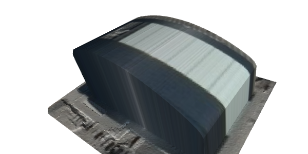During the third edition of FOSS4G Belgium We gave an interactive demo of point cloud processing techniques at the third edition of FOSS4G Belgium 2017 and at FOSDEM 2018. Both conferences promote free and open source software and accordingly the demo is available both as a static webpage, and as a github repo. Here’s an overview of the demo, hopefully shedding some light on how you too can play and interact with 3D point clouds in a Jupyter notebook using python, pdal and ipyvolume.

Before talking data processing, let’s talk data. The dataset we’re interested in comes in the form of a 3D point cloud, i.e. a long list of points with X, Y and Z coordinates (and some metadata). In this case, it corresponds to about 16 points per square meter covering the whole of Flanders and Brussels. This open data set from the Flemish Government was collected between 2013 and 2015 using airborne lidar sensors.

Tree modelling

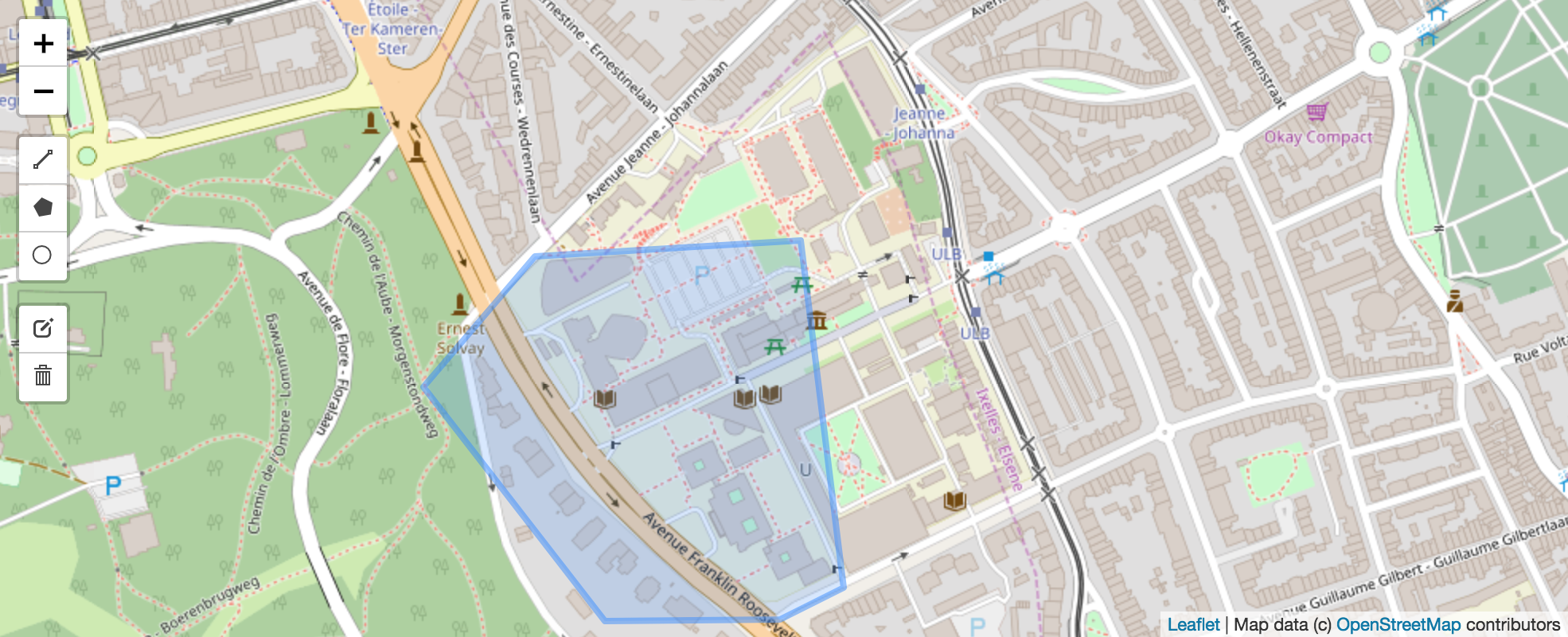
The first part of the demo focusses on points in the street outside the conference building, selected by drawing live a polygon in an ipyleaflet widget.

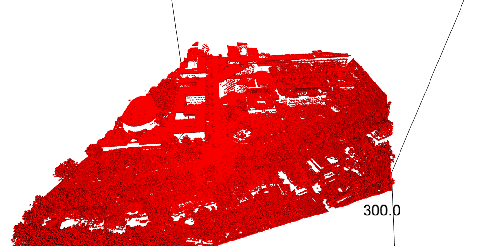
These points are placed irregularly in space, and the first step in processing such data consists in comparing a point with its closest neighbours. For example, do all neighbours look planar? Is this plane horizontal? Are all nearby points rougly at the same level or above? Answering these questions is the basis for separating points which are on the ground from those which aren’t. Points already come equipped with the result of such an algorithm, so we don’t need to worry about that.

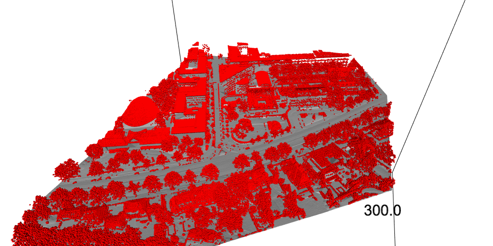
Looking at the remaining points looks like a mess, but moving those points around in 3D we see two main types of objects: trees and buildings. In order to separate between the two, we compute a measure of flatness of the neighbouring points and set a threshold. As seen below, this already does a good job at separating trees from buildings. Up to here, all the processing is handled by PDAL, a big favorite of ours.

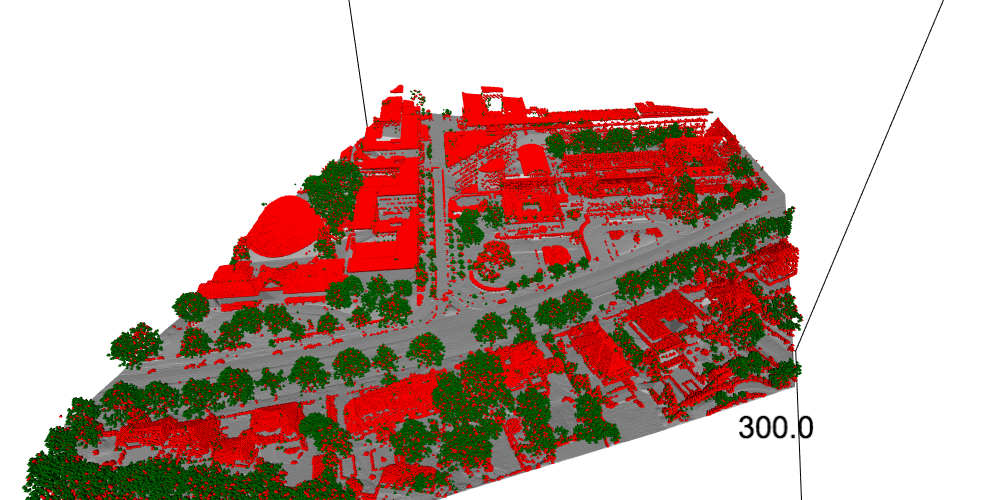
The next step is to identify individual trees. One way to achieve this is to look for treetops, geometrically identified as those points which are the highest among all their neighbours.

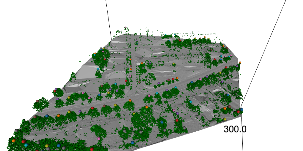
Finally trees are differentiated in terms of the closest treetop, which in turn allows to roughly model what the trees look like using spheres.

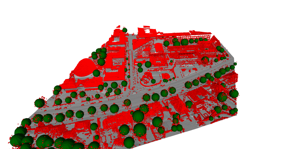
Here’s a video summing up the whole process.

Building modelling

In the second part of the demo, we build a 3D model of the conference building in relatively few lines of codes. As before, we use ipyleaflet to select the points on and around the building.

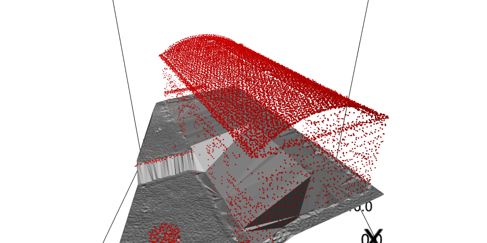
Although the building is complex and there may be some missing data, it is easy to model because:

1. it is rectangular viewed from above;
2. the shape of the roof is determined by its view from the side.

Given those two facts, all we need to model the building is to determine its orientation in the horizontal plane. This is where we pull a magic trick in the form of normals vectors, conveniently provided by our faithful preprocessor PDAL. Each flat neighbourhood is perpendicular to a normal vector, and the collection of those normal vectors point mostly in a specific direction.

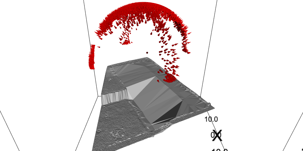
Identify this direction, rotate the building to align it to the X and Y axes…

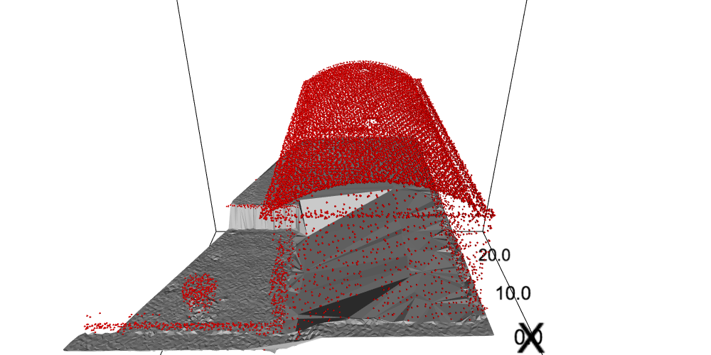
…and you’re almost done building a 3D model.

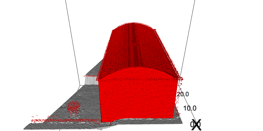
Finally, we rotate back the model to the original coordinates and apply texture from aerial imagery, which finished the trick.

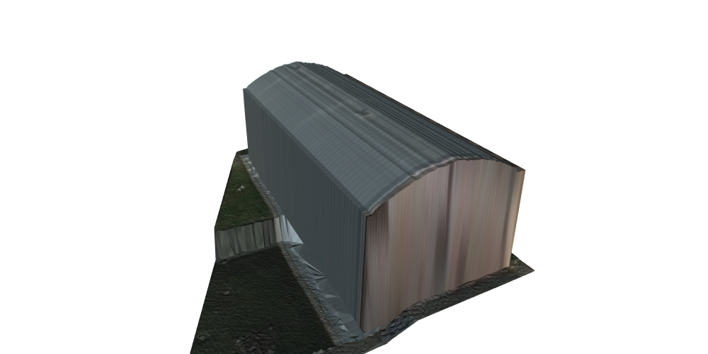
Here’s a quick video version of the processing.

Ok, maybe that was a bit fast, but remember that all the code is available on github and now it’s

Your turn to play

Clone the repository, Install a Jupyter / python / pdal stack using conda by following the instructions, and start doing some point cloud processing too!

Advanced modelling

Interested in more advanced 3D modelling of buildings? Check out the demo of our 3D models for every building in Flanders.